Conducting Reliable Mineral Resource Investigations: A Comprehensive Technical Guide Aligned with SNI 4726-2019

Executive Summary

This technical report provides a comprehensive framework for conducting mineral resource investigations that produce reliable estimates compliant with the Indonesian National Standard for Reporting Exploration Results, Mineral Resources, and Mineral Reserves (SNI 4726-2019). The report synthesizes international best practices with Indonesian regulatory requirements to address three critical objectives: (1) establishing rigorous investigation methodologies encompassing sampling protocols, data quality assurance, geological modeling, and estimation techniques; (2) identifying frequently overlooked errors that compromise estimate reliability despite appearing technically sound; and (3) providing detailed inspection checklists aligned with SNI 4726-2019 to ensure accuracy and defensibility.

Key findings indicate that reliable mineral resource estimates require disciplined sampling with robust quality assurance/quality control (QA/QC) programs, clear geological domain definition, appropriate change-of-support corrections, and honest statistical validation [1]. Many superficially correct models conceal critical flaws including sampling bias, improper compositing, domain boundary errors, or misuse of kriging variance for uncertainty quantification [1]. The report demonstrates that systematic application of verification protocols—covering data integrity, assay QA/QC, compositing strategy, geological model validation, variography diagnostics, and uncertainty quantification—is essential for producing estimates that meet SNI 4726-2019 requirements and international reporting standards.

This guide is designed for mining professionals, competent persons, and technical reviewers responsible for mineral resource estimation and reporting in Indonesia. It provides actionable procedures, critical control points, and decision criteria to ensure that exploration results translate into reliable, defensible mineral resource estimates suitable for investment decisions and regulatory compliance.

1. Introduction

Mineral resource estimation is a critical technical and economic activity that underpins investment decisions, mine planning, and regulatory compliance in the mining industry. In Indonesia, the Indonesian National Standard SNI 4726-2019 establishes mandatory requirements for reporting exploration results, mineral resources, and mineral reserves, aligning national practice with international standards such as the JORC Code (2012), CIM Definition Standards (2014), and SAMREC Code (2016). Despite the availability of sophisticated geostatistical software and standardized reporting frameworks, mineral resource estimates frequently contain significant errors that remain undetected until production reconciliation reveals substantial discrepancies [1], [3].

The consequences of unreliable resource estimates extend beyond technical embarrassment. Overestimated resources can lead to uneconomic mine designs, stranded capital investments, and regulatory sanctions, while underestimated resources result in missed economic opportunities and suboptimal extraction strategies [12]. Research indicates that sampling errors and estimation biases can introduce 10-50% variance in resource tonnage and grade estimates, with cumulative effects potentially rendering projects economically unviable [15]. The challenge is compounded by the fact that many errors are systematically concealed within technically sophisticated workflows that superficially appear compliant with best practices [3].

This report addresses three fundamental questions that confront mining professionals and competent persons responsible for mineral resource estimation in Indonesia:

1. What constitutes a rigorous investigation methodology that ensures data quality, geological understanding, and statistical validity throughout the resource estimation workflow?
2. What are the most frequently overlooked errors that compromise estimate reliability despite superficial compliance with technical standards and reporting codes?
3. What inspection protocols and verification checklists should be systematically applied to ensure that mineral resource estimates meet SNI 4726-2019 requirements and are defensible under technical and regulatory scrutiny?

The report synthesizes international best practices with Indonesian regulatory requirements to provide actionable guidance for conducting reliable mineral resource investigations. Section 2 establishes the regulatory context and SNI 4726-2019 framework. Section 3 presents a comprehensive investigation methodology covering sampling, QA/QC, compositing, geological modeling, variography, estimation, and validation. Section 4 identifies frequently covered-up errors that escape routine quality checks. Section 5 provides detailed inspection checklists aligned with SNI 4726-2019 requirements. The report is designed to serve as both a technical reference for practitioners and a verification tool for reviewers and competent persons.

---

2. Regulatory Framework and SNI 4726-2019 Context

2.1 Indonesian National Standard SNI 4726-2019

The Indonesian National Standard SNI 4726-2019, titled “Pelaporan Hasil Eksplorasi, Sumber Daya Mineral, dan Cadangan Mineral” (Reporting of Exploration Results, Mineral Resources, and Mineral Reserves), establishes mandatory requirements for public reporting of exploration results and resource/reserve estimates in Indonesia. Promulgated by the National Standardization Agency (Badan Standardisasi Nasional, BSN) and enforced by the Ministry of Energy and Mineral Resources, SNI 4726-2019 aligns Indonesian practice with international reporting standards while incorporating specific requirements relevant to Indonesian geological settings and regulatory frameworks [4].

SNI 4726-2019 adopts the fundamental definitions and classification framework established by international codes, including:

• Exploration Results: Data and information generated by mineral exploration programs, including geological observations, geophysical surveys, geochemical analyses, and drilling results, that have not yet been classified as mineral resources.
• Mineral Resources: Concentrations or occurrences of material of economic interest in or on the Earth’s crust in such form, grade, and quantity that there are reasonable prospects for eventual economic extraction. Mineral resources are subdivided into Inferred, Indicated, and Measured categories based on increasing levels of geological confidence.
• Mineral Reserves: The economically mineable part of a Measured or Indicated Mineral Resource, demonstrated by at least a Preliminary Feasibility Study. Mineral reserves are subdivided into Probable and Proven categories.

The standard emphasizes that mineral resource and reserve estimates must be prepared by or under the supervision of a Competent Person (Orang yang Berkompeten, OyB)—a minerals industry professional with relevant education, experience, and membership in a recognized professional organization who is subject to enforceable professional codes of ethics [1]. The Competent Person must take responsibility for the technical content and conclusions of public reports, ensuring that estimates are based on adequate data, appropriate methodologies, and realistic assumptions.

2.2 Key Requirements and Compliance Obligations

SNI 4726-2019 establishes specific requirements that directly impact mineral resource investigation methodologies:

Data Quality and Documentation: All exploration data used for resource estimation must be collected using industry-standard methods with documented quality assurance and quality control (QA/QC) procedures. The standard requires disclosure of sampling methods, sample preparation procedures, analytical techniques, QA/QC protocols, and data verification procedures [1]. Competent Persons must verify that data quality is adequate to support the level of confidence assigned to resource classifications.

Geological Understanding: Resource estimates must be based on a sound geological model that explains the spatial distribution, geometry, and continuity of mineralization. The standard requires documentation of geological interpretations, including lithological units, structural controls, alteration patterns, and mineralization styles [9]. Domain boundaries must be geologically justified and validated against drilling data.

Estimation Methodology: The choice of estimation method (e.g., inverse distance weighting, ordinary kriging, indicator kriging) must be appropriate for the deposit type, data density, and grade distribution characteristics. The standard requires documentation of estimation parameters, including search strategies, compositing methods, top-cutting procedures, and block size selection [6]. Geostatistical methods must be supported by variography that demonstrates spatial continuity.

Classification Criteria: The classification of mineral resources into Inferred, Indicated, and Measured categories must reflect geological confidence, data density, and estimation uncertainty. SNI 4726-2019 requires that classification criteria be clearly defined, consistently applied, and validated against estimation quality metrics [8]. The standard emphasizes that kriging variance alone is insufficient for classification and must be supplemented by geological judgment and validation against drilling density.

Validation and Reconciliation: Resource estimates must be validated using multiple independent methods, including visual inspection, statistical comparison with input data, and cross-validation techniques. Where production data are available, estimates must be reconciled against actual mining results to demonstrate predictive accuracy [12].

2.3 Alignment with International Reporting Standards

SNI 4726-2019 is explicitly designed to align with international reporting standards, particularly the JORC Code (2012 Edition), CIM Definition Standards (2014), and SAMREC Code (2016). This alignment facilitates international investment, enables dual listing on Indonesian and foreign stock exchanges, and ensures that Indonesian resource estimates are recognized and accepted by international financial institutions and mining companies [19].

The standard adopts the international principle of Reasonable Prospects for Eventual Economic Extraction (RPEEE), which requires that mineral resources be reported only where there is a reasonable expectation that mineralization could be economically extracted under realistic assumptions about mining methods, metallurgical recovery, commodity prices, and operating costs [19]. This principle prevents the reporting of geologically interesting but economically irrelevant mineralization as mineral resources.

SNI 4726-2019 also incorporates the international emphasis on transparency, materiality, and competence as the three pillars of reliable resource reporting. Public reports must provide sufficient information for a reasonably informed reader to understand the basis of the estimate, the key assumptions and limitations, and the level of confidence that can be placed in the reported figures [8].

2.4 Implications for Investigation Methodology

The requirements of SNI 4726-2019 have direct implications for the design and execution of mineral resource investigations:

1. Systematic QA/QC Programs: The standard’s emphasis on data quality necessitates the implementation of comprehensive QA/QC programs that include field duplicates, certified reference materials, blank samples, and laboratory performance monitoring [11].
2. Geological Model Validation: The requirement for geologically justified domain boundaries demands rigorous validation of geological interpretations against drilling data, geophysical surveys, and metallurgical test work [9].
3. Appropriate Estimation Methods: The standard’s requirement for methodology appropriateness necessitates careful evaluation of estimation techniques relative to deposit characteristics, data distribution, and grade continuity [6].
4. Transparent Documentation: The emphasis on transparency requires detailed documentation of all investigation procedures, assumptions, limitations, and validation results in a format that supports independent technical review [8].

The following sections present a comprehensive investigation methodology designed to meet these requirements and produce mineral resource estimates that are technically sound, defensible, and compliant with SNI 4726-2019.

---

3. Investigation Methodology for Reliable Mineral Resource Estimation

This section presents a systematic methodology for conducting mineral resource investigations that produce reliable, defensible estimates compliant with SNI 4726-2019. The methodology encompasses seven critical components: sampling and field data collection, laboratory analysis and QA/QC programs, sample support and compositing strategy, geological modeling and domain definition, variography and spatial statistics, estimation methods and techniques, and validation and classification. Each component is addressed with specific procedures, critical control points, and quality criteria.

3.1 Sampling and Field Data Collection

Sampling is the foundation of mineral resource estimation, and sampling errors propagate through all subsequent stages of the estimation workflow. Research indicates that sampling errors can contribute 30-60% of total estimation variance, making sampling methodology the single most important determinant of estimate reliability [15]. SNI 4726-2019 requires that sampling methods be appropriate for the material being sampled, the mineralization style, and the intended use of the data [1].

3.1.1 Drilling Methods and Sample Collection

The selection of drilling method (diamond core drilling, reverse circulation drilling, or rotary air blast drilling) must be appropriate for the deposit type, geological conditions, and required sample quality. Diamond core drilling provides the highest quality samples and enables detailed geological logging, structural measurements, and geotechnical characterization, making it the preferred method for resource definition drilling in most deposit types [1]. Reverse circulation (RC) drilling is cost-effective for reconnaissance exploration and grade control in oxidized or unconsolidated materials but may introduce sample contamination or loss in competent rock.

Figure 1: Mineral Exploration Drilling and Core Sampling Technical Overview

This comprehensive diagram illustrates the complete drilling and sampling workflow for mineral resource investigations. The plan view (top left) shows systematic grid drilling patterns and infill drilling strategies used to achieve appropriate data density for resource classification. The subsurface cross-section (bottom left) demonstrates drill hole trajectories through geological units, including overburden, weathered bedrock, mineralized zones, waste rock, and deep basement rock, with core sample collection zones marked at regular intervals. The right panel details the core sampling process, including drill string assembly with diamond coring bits, core barrel and sample extraction procedures, and the core box logging station where geologists perform sample labeling, geological logging, and systematic documentation.

The diagram emphasizes the importance of maintaining 95% core recovery in mineralized zones and implementing proper chain-of-custody protocols from drill site to laboratory. This systematic approach to drilling and sampling forms the foundation for reliable mineral resource estimation by ensuring representative, unbiased sample collection with complete documentation.

Critical sampling protocols include:

Sample Interval Selection: Sample intervals should be selected to honor geological boundaries while maintaining sufficient sample support for statistical analysis. Variable-length sampling that respects lithological contacts is generally superior to fixed-length sampling that arbitrarily cuts across geological boundaries [2]. However, extreme length variations (e.g., 0.3 m to 5 m intervals) complicate compositing and require careful change-of-support corrections [14].

Sample Recovery and Representativeness: Core recovery must be measured and documented for all drill holes, with particular attention to recovery in mineralized zones. Low recovery (<85%) in mineralized intervals may indicate sample loss of friable, high-grade material, introducing negative bias into resource estimates [15]. Competent Persons must evaluate whether low recovery is random or systematically associated with specific lithologies or grade ranges.

Sample Contamination and Cross-Contamination: Drilling procedures must minimize sample contamination from drilling fluids, cuttings from overlying intervals, or residual material in sampling equipment. RC drilling is particularly susceptible to contamination from wet samples or inadequate cyclone cleaning between intervals [15]. Systematic insertion of blank samples in the analytical stream can detect and quantify contamination.

Geological Logging and Documentation: All drill core must be geologically logged by qualified geologists using standardized logging codes and procedures. Logging should capture lithology, alteration, mineralization style, structure, weathering, and other features relevant to geological modeling and domain definition [1]. Digital logging systems with photographic core documentation provide permanent records that support subsequent reinterpretation.

Sample Security and Chain of Custody: Samples must be securely stored and transported with documented chain-of-custody procedures to prevent tampering, loss, or sample switching. SNI 4726-2019 requires disclosure of sample security measures, particularly for high-value commodities where the risk of tampering is elevated [1].

3.1.2 Sampling Bias and Representativeness

Sampling bias—systematic deviation of sample grades from true in-situ grades—is one of the most insidious sources of estimation error because it is difficult to detect and correct retrospectively [15]. Common sources of sampling bias include:

Selective Sampling: Preferential sampling of visibly mineralized intervals while avoiding barren or low-grade zones introduces positive bias. This practice, sometimes called “high-grading the drill core,” can inflate resource estimates by 20-50% [3]. Competent Persons must verify that sampling protocols require complete sampling of all intervals within defined mineralized domains, regardless of visual appearance.

Sample Loss During Drilling: Differential loss of friable, high-grade material during drilling introduces negative bias. This is particularly problematic in oxide zones, weathered rock, and fault zones where competent material is preferentially recovered while friable material is lost as fines [15].

Sample Preparation Bias: Crushing, splitting, and pulverizing procedures can introduce bias if coarse high-grade particles are preferentially lost or retained. The “nugget effect” in coarse gold deposits is often exacerbated by inadequate sample preparation protocols that fail to achieve representative subsampling [15].

Analytical Bias: Systematic analytical errors due to matrix effects, incomplete digestion, or instrument drift introduce bias that affects all samples processed during a particular period. Regular insertion of certified reference materials (CRMs) is essential for detecting and correcting analytical bias [11].

The diagram in Figure 1 illustrates proper drilling and sampling procedures designed to minimize these sources of bias, including systematic grid patterns, complete core recovery documentation, and rigorous sample handling protocols.

3.2 Laboratory Analysis and QA/QC Programs

Laboratory analysis converts physical samples into numerical grade data that form the basis of resource estimation. The reliability of analytical data depends on appropriate analytical methods, rigorous quality control procedures, and systematic monitoring of laboratory performance. SNI 4726-2019 requires disclosure of analytical methods, detection limits, QA/QC protocols, and data verification procedures [1].

3.2.1 Analytical Methods and Detection Limits

The selection of analytical method must be appropriate for the commodity, expected grade range, and mineralogical characteristics. Common analytical methods include:

Fire Assay: The industry standard for gold and platinum group elements, fire assay provides accurate results across a wide grade range (0.01 g/t to >100 g/t) and is relatively insensitive to mineralogical variations [1]. However, fire assay is destructive, expensive, and subject to nugget effect in coarse gold deposits.

Multi-Element ICP-MS/ICP-AES: Inductively coupled plasma mass spectrometry (ICP-MS) and atomic emission spectrometry (ICP-AES) provide rapid, cost-effective multi-element analysis suitable for base metals, rare earth elements, and pathfinder elements. These methods require complete sample digestion (four-acid or fusion digestion) to avoid matrix effects and incomplete recovery [1].

X-Ray Fluorescence (XRF): Portable and laboratory XRF provides rapid, non-destructive analysis suitable for grade control and preliminary exploration. However, XRF is subject to matrix effects, requires careful calibration, and may not achieve the precision required for resource estimation [1].

Detection limits must be appropriate for the expected grade range and economic cutoff grades. Analytical methods with detection limits above the cutoff grade are unsuitable for resource estimation because they cannot distinguish economic from sub-economic material [1].

3.2.2 Quality Assurance and Quality Control Protocols

Robust QA/QC programs are essential for detecting analytical errors, monitoring laboratory performance, and ensuring data reliability. SNI 4726-2019 requires that QA/QC protocols include certified reference materials, blank samples, field duplicates, and laboratory duplicates at frequencies sufficient to provide statistical confidence in data quality [1], [11].

Figure 2: Mineral Resource Estimation QAQC Quality Control Process

This comprehensive flowchart illustrates the complete quality assurance and quality control workflow for mineral resource estimation, from initial sample collection through final database approval. The process begins with field sample collection and chain-of-custody documentation, followed by two-stage sample preparation (drying, crushing, riffle splitting, then fine grinding, homogenization, and sub-sampling). Three QA/QC insertion points are strategically placed throughout the workflow:

(1) field duplicates inserted every 20th sample during collection,

(2) certified reference materials (CRMs) inserted at a rate of 1 in 20 during preparation, and

(3) blank samples (1 in 20) and laboratory duplicates (1 in 20) inserted before assay analysis.

Following fire assay or ICP-MS/XRF multi-element analysis, the data undergoes rigorous validation through multiple decision points: CRM results must fall within acceptable limits (±2SD), blank results must be below detection limits, and field/lab duplicates must show acceptable precision (HARD <20%). Statistical validation includes outlier detection, grade distribution analysis, and spatial continuity checks.

Geological validation cross-checks results against lithology and geological models, verifying mineralization patterns. If any validation check fails, corrective actions are triggered, including sample re-assay, investigation of laboratory procedures, review of geological interpretations, or consultation with geologists.

Only after all QA/QC criteria are met and senior geologist/qualified person approval is obtained is the database locked for resource estimation. This systematic approach ensures data integrity and compliance with SNI 4726-2019 requirements.

Certified Reference Materials (CRMs): CRMs are commercially prepared standards with certified grade values and statistical confidence intervals. CRMs should be inserted into the sample stream at a frequency of 1 in 20 samples (5%) and should span the expected grade range of the deposit [11]. CRM results are evaluated using control charts that plot measured values against certified values with ±2 standard deviation control limits. Results outside control limits indicate analytical bias or precision problems requiring corrective action.

Blank Samples: Blank samples (barren material with grades below detection limits) are inserted to detect sample contamination or carryover from high-grade samples. Blanks should be inserted at a frequency of 1 in 20 samples, with additional blanks inserted immediately following high-grade samples [11]. Blank failures (grades above detection limits) indicate contamination in sample preparation or analytical procedures.

Field Duplicates: Field duplicates are collected by splitting drill core or RC samples in the field using riffle splitters or cone-and-quarter methods. Field duplicates assess the combined variability of sampling, sample preparation, and analysis. The Half Absolute Relative Difference (HARD) between duplicate pairs should be <20% for 90% of pairs; higher HARD values indicate inadequate sample preparation or excessive nugget effect [11].

Laboratory Duplicates: Laboratory duplicates are prepared by splitting pulverized samples and analyzing both splits. Laboratory duplicates assess analytical precision and sample preparation variability. HARD values for laboratory duplicates should be <10% for 90% of pairs [11].

The flowchart in Figure 2 illustrates the complete QA/QC workflow, including insertion points for quality control samples, validation decision points, and corrective actions triggered by QA/QC failures. This systematic approach ensures that only data meeting stringent quality criteria are used for resource estimation.

3.2.3 Data Validation and Database Management

Raw analytical data must be validated and loaded into a secure, auditable database that maintains data integrity and traceability. Data validation procedures include:

Coordinate Verification: Drill hole collar coordinates must be surveyed using differential GPS or total station methods with accuracy appropriate for the drill spacing and deposit size. Downhole survey data (azimuth and dip measurements) must be collected at regular intervals (typically 30 m) using gyroscopic or magnetic survey tools [1].

Assay Database Integrity: Assay data must be checked for transcription errors, missing intervals, overlapping intervals, and out-of-sequence samples. Automated database validation scripts can detect common errors such as negative assay values, grades exceeding physically plausible limits, or sample intervals extending beyond drill hole depth [1].

Geological Consistency: Assay grades must be cross-checked against geological logging to verify that high grades occur in expected lithologies and mineralization styles. Anomalous grades in barren lithologies may indicate sample mix-ups or labeling errors [3].

3.3 Sample Support and Compositing Strategy

Sample support—the physical volume and geometry of material represented by a sample—has profound implications for resource estimation. Raw assay data typically represent variable-length intervals (0.5 m to 3 m) that must be composited into uniform-length intervals for geostatistical analysis and block model estimation. Improper compositing introduces bias, distorts grade distributions, and invalidates variography [2], [14].

3.3.1 Compositing Methods and Length Selection

Compositing combines variable-length assay intervals into uniform-length composites using length-weighted averaging. The composite length should be selected based on:

• Minimum mining selectivity: The smallest volume that can be selectively mined and processed. For underground mining, this is typically 1-2 m; for open pit mining, 5-10 m [2].
• Geological continuity: Composite length should be small enough to honor geological boundaries and grade trends but large enough to provide stable statistics [2].
• Data density: Composite length should be compatible with drill hole spacing. As a rule of thumb, composite length should be 1/3 to 1/2 of the drill spacing [2].

Figure 3: Compositing and Change of Support in Mineral Resource Estimation

This comprehensive diagram illustrates the critical concepts of sample compositing and changes of support in mineral resource estimation. The top-left panel shows the sample compositing process, where variable-length drill core samples (ranging from 0.5m at 2.3 g/t to 1.5m at 3.5 g/t) are transformed into uniform 1m composites using length-weighted averaging:

Composite Grade = Σ(Sample Grade × Sample Length) / Σ(Sample Length). This process standardizes data for geostatistical analysis while preserving total metal content. The top-right panel illustrates the fundamental difference between point support (individual core samples with high variability, grades ranging from 1.5 g/t to 4.2 g/t) and block support (averaged block grades of 2.8 g/t representing 10m × 10m × 5m volumes). The bottom-left panel demonstrates change of support correction, showing how point grade distribution (red histogram, mean = 2.5 g/t, σ²sample = 2.5) is transformed into block grade distribution (blue histogram, mean = 2.5 g/t, σ²block = 0.8) through the variance reduction factor f = σ²block / σ²sample < 1.

This correction is essential for realistic resource estimation because block grades are inherently less variable than point samples due to spatial averaging. The bottom-right panel compares kriged point estimates (left, showing high variability with many high-grade spots) versus block model estimates (right, showing smoothed grades with reduced extremes), illustrating the smoothing effect inherent in block kriging. The grade scale ranges from blue (0-2 g/t) through green (2-4 g/t) and yellow (4-6 g/t) to red (8-10 g/t). This diagram emphasizes that proper compositing and change of support corrections are essential for producing realistic, unbiased resource estimates that reflect the true variability of block grades rather than point sample grades.

Length-Weighted Compositing: The standard compositing method uses length-weighted averaging:

Composite Grade=∑i=1n(gi×li)∑i=1nliComposite Grade=∑i=1nli∑i=1n(gi×li)

where $g_i$ is the grade of interval $i$, $l_i$ is the length of interval $i$, and $n$ is the number of intervals in the composite [2].

Top-Cutting and Capping: High-grade outliers (often called “nuggets”) can dominate length-weighted composites and introduce positive bias. Top-cutting restricts individual interval grades to a maximum value before compositing, while capping restricts composite grades after compositing. The top-cut threshold should be selected using statistical methods (e.g., probability plots, coefficient of variation analysis) and validated by examining the spatial distribution of high grades [3].

Residual Intervals and Boundary Composites: Intervals at the top or bottom of mineralized zones that are shorter than the composite length (residual intervals) require special treatment. Options include: (1) combining residuals with adjacent composites if the length difference is small (<30%), (2) retaining residuals as short composites if they represent genuine geological boundaries, or (3) discarding residuals if they are artifacts of arbitrary sampling intervals [2].

The diagram in Figure 3 illustrates the compositing process, showing how variable-length samples (0.5m to 1.5m) are transformed into uniform 1m composites using length-weighted averaging. The diagram emphasizes that proper compositing preserves total metal content while standardizing data for geostatistical analysis.

3.3.2 Change of Support and Block Variance

A fundamental principle of geostatistics is that block grades (the volume-averaged grade of a mining block) are less variable than point sample grades due to spatial averaging within the block volume. This phenomenon, called “change of support,” means that the variance of block grades is systematically lower than the variance of point sample grades [14].

Failure to account for change of support leads to overestimation of high-grade blocks and underestimation of low-grade blocks, a problem known as “conditional bias” [7]. While some conditional bias is inevitable in kriging, excessive bias indicates inadequate change-of-support correction or inappropriate estimation parameters [7].

Variance Reduction Factor: The relationship between point variance ($\sigma^2_{\text{point}}$) and block variance ($\sigma^2_{\text{block}}$) is quantified by the variance reduction factor:

f=σblock2σpoint2<1f=σpoint2σblock2<1

The variance reduction factor depends on block size, variogram parameters, and the spatial configuration of samples within blocks. Larger blocks have smaller variance reduction factors (more smoothing), while smaller blocks approach point variance [14].

Change-of-Support Corrections: Several methods exist for correcting point estimates to block support:

1. Affine Correction: A simple linear transformation that adjusts the mean and variance of point estimates to match expected block statistics [14].
2. Indirect Lognormal Correction: Assumes lognormal grade distribution and uses analytical formulas to transform point estimates to block support [14].
3. Discrete Gaussian Model: A non-parametric method that transforms point grades to Gaussian space, performs block kriging, and back-transforms to original units with change-of-support correction [14].

The bottom panels of Figure 3 illustrate change of support effects, showing how point grade distribution (red histogram, high variance) is transformed into block grade distribution (blue histogram, lower variance) through the variance reduction factor. The right panels compare kriged point estimates (high variability, many extreme values) versus block model estimates (smoothed grades, reduced extremes), demonstrating the smoothing effect inherent in block kriging.

3.3.3 Compositing Within Geological Domains

Compositing should respect geological domain boundaries to avoid diluting high-grade domains with low-grade material or vice versa. Two approaches are commonly used:

Domain-Restricted Compositing: Composites are created separately within each geological domain, with composites truncated at domain boundaries. This approach preserves domain integrity but creates variable-length composites at boundaries [2].

Boundary Composites: Composites that straddle domain boundaries are assigned to the domain containing the majority of the composite length, or are split into separate composites for each domain. The choice depends on the sharpness of domain boundaries and the grade contrast between domains [2].

3.4 Geological Modeling and Domain Definition

Geological modeling—the three-dimensional representation of lithology, structure, alteration, and mineralization—is the framework within which resource estimation is conducted. SNI 4726-2019 requires that resource estimates be based on a sound geological model that explains the spatial distribution and continuity of mineralization [1], [9].

3.4.1 Geological Domain Definition

Geological domains are volumes of rock with relatively homogeneous geological and grade characteristics that can be estimated separately. Domain definition is one of the most critical and subjective steps in resource estimation, as inappropriate domains can introduce significant bias [9].

Domain Definition Criteria: Domains should be defined based on:

• Lithology: Different rock types often have distinct mineralization styles and grade distributions.
• Alteration: Alteration assemblages (e.g., potassic, phyllic, argillic) often correlate with metal grades and mineralogy.
• Mineralization style: Vein-hosted, disseminated, and replacement mineralization require different estimation approaches.
• Structural controls: Faults, folds, and shear zones control mineralization geometry and continuity.
• Weathering: Oxide, transition, and fresh rock zones have different metallurgical characteristics and grade distributions [9].

Hard Boundaries vs. Soft Boundaries: Hard boundaries (e.g., lithological contacts, faults) are treated as impermeable during estimation, preventing samples from one domain from influencing estimates in adjacent domains. Soft boundaries allow limited cross-domain estimation where geological transitions are gradational [9].

Domain Validation: Geological domains must be validated by demonstrating that:

• Within-domain grade distributions are more homogeneous than the global grade distribution.
• Domain boundaries align with observable geological features in drill core and outcrop.
• Domains have sufficient data density to support independent estimation [9].

3.4.2 Wireframe Modeling and Implicit Modeling

Geological domains are represented as three-dimensional wireframe surfaces or implicit models:

Wireframe Modeling: Traditional approach where geologists manually digitize domain boundaries on cross-sections, then connect sections to create 3D wireframe surfaces. Wireframes provide explicit control over domain geometry but are labor-intensive and subject to interpretation bias [1].

Implicit Modeling: Automated approach that uses interpolation algorithms (e.g., radial basis functions) to generate smooth domain surfaces from interpreted points or strings. Implicit modeling is faster and more reproducible than wireframe modeling but may create geologically unrealistic surfaces if input data are sparse or inconsistent [1].

Validation Against Drilling: Domain models must be validated by comparing predicted domain boundaries against actual geological contacts observed in drill holes. Significant discrepancies indicate that the domain model requires revision [9].

3.4.3 Block Model Framework

The block model is a three-dimensional array of rectangular blocks (cells) that discretizes the deposit volume. Each block is assigned estimated grades, geological codes, and classification categories. Block model design parameters include:

Block Size: Block dimensions should reflect the minimum mining selectivity and data density. Typical block sizes range from 5m × 5m × 5m for underground deposits to 25m × 25m × 10m for large open pit deposits [6]. Blocks should be small enough to honor geological boundaries but large enough to be supported by available data.

Block Discretization: Large blocks may be subdivided into smaller sub-blocks (e.g., 2m × 2m × 2m) near domain boundaries to improve volume calculations and honor complex geological shapes. Sub-blocks are estimated using the same parameters as parent blocks [6].

Model Extent and Rotation: The block model should extend beyond the current drilling envelope to accommodate future exploration. Model rotation should align with the principal directions of mineralization continuity (determined from variography) to optimize estimation efficiency [6].

3.5 Variography and Spatial Statistics

Variography quantifies the spatial continuity of mineralization—how rapidly grades change with distance and direction. Variogram parameters control the weighting of samples during kriging and directly determine the smoothness and reliability of grade estimates. SNI 4726-2019 requires that geostatistical estimation methods be supported by variography that demonstrates spatial continuity [1].

3.5.1 Experimental Variogram Calculation

The experimental variogram measures the average squared difference between sample pairs separated by a given distance (lag) and direction:

γ(h)=12N(h)∑i=1N(h)[Z(xi)−Z(xi+h)]2γ(h)=2N(h)1∑i=1N(h)[Z(xi)−Z(xi+h)]2

where $\gamma(h)$ is the semivariance at lag distance $h$, $Z(x_i)$ is the grade at location $x_i$, and $N(h)$ is the number of sample pairs separated by distance $h$ [1].

Figure 4: Variogram Analysis and Spatial Continuity in Mineral Resource Estimation

This comprehensive diagram illustrates the fundamental concepts and practical application of variogram analysis for quantifying spatial continuity in mineral deposits. The top-left panel shows an experimental variogram with lag distance plot, displaying the mathematical formula γ(h) = ½E[(Z(x+h) – Z(x))²] and key components: nugget effect (C₀) representing micro-scale variability and measurement error, partial sill (C) representing structural spatial variance, and total sill (C₀+C) representing total variance.

The range (a) indicates the distance beyond which samples are spatially uncorrelated. The top-center panel breaks down variogram model components and presents three standard theoretical models: Spherical model α = C₀[Z(x+h) – a²], Exponential model C = C(e^(-h/a²)), and Gaussian model α = C₀(e^(-(x+h)/a)). The top-right panel displays a 2D variogram heat map showing spatial continuity patterns, with the major axis of continuity (150m range) and minor axis of continuity (80m range) clearly marked, indicating anisotropic mineralization geometry. The bottom-left panel presents directional variograms showing anisotropy, with the 0° major direction (range = 150m, red curve) exhibiting greater continuity than the 90° minor direction (range = 80m, blue curve), yielding an anisotropy ratio of Major/Minor = 150m/80m = 1.875.

The bottom-center panel illustrates the 3D search ellipsoid representation with major axis (a₁ = 100m), semi-major axis (a₂ = 80m), and minor axis (a₃ = 40m), oriented at azimuth (α), dip (β), and plunge (γ) angles. Experimental scatter points and model fit curves with confidence intervals (shaded areas) demonstrate proper variogram modeling. The bottom-right panel shows the 2D plan view of the search ellipsoid with azimuth = 45° and clearly marked major axis (150m) and minor axis (80m). This diagram emphasizes that proper variogram analysis is essential for understanding spatial continuity patterns, determining appropriate search parameters for kriging, and ensuring that estimation honors the geological structure and anisotropy of the mineral deposit.

Variogram Parameters: The experimental variogram is characterized by three key parameters:

• Nugget Effect ($C_0$): The discontinuity at the origin, representing micro-scale variability, measurement error, and sampling error. High nugget effects (>50% of total sill) indicate poor spatial continuity or data quality problems [1].
• Sill ($C_0 + C$): The plateau value that the variogram approaches at large distances, approximately equal to the data variance. The structural component ($C$) represents spatially correlated variability [1].
• Range ($a$): The distance at which the variogram reaches the sill, representing the correlation length. Sample pairs separated by distances greater than the range are spatially uncorrelated [1].

The top-left panel of Figure 4 shows an experimental variogram with these components clearly labeled, demonstrating how semivariance increases with lag distance until reaching the sill at the range distance.

3.5.2 Variogram Modeling and Anisotropy

Experimental variograms are fitted with theoretical variogram models (spherical, exponential, or Gaussian) that provide smooth, continuous functions for kriging calculations. The choice of model type affects the shape of the kriging weights and the degree of smoothing [1].

Anisotropy: Most mineral deposits exhibit anisotropic spatial continuity—grades are more continuous in some directions (e.g., along strike or bedding) than others (e.g., across strike or perpendicular to bedding). Anisotropy is quantified by calculating directional variograms in multiple directions and comparing their ranges [1].

The bottom-left panel of Figure 4 shows directional variograms demonstrating anisotropy, with the 0° major direction (red curve, range = 150m) exhibiting greater continuity than the 90° minor direction (blue curve, range = 80m). The anisotropy ratio of 1.875 indicates that mineralization is nearly twice as continuous along strike as across strike.

Search Ellipsoid: Anisotropic variogram parameters define the search ellipsoid used during kriging—an ellipsoidal search volume oriented along the principal directions of continuity. The search ellipsoid dimensions are typically set to 1.5-2.0 times the variogram ranges in each direction [6]. The bottom-center and bottom-right panels of Figure 4 illustrate the 3D search ellipsoid and its 2D plan view projection, showing how the ellipsoid is oriented at azimuth 45° with major axis 150m and minor axis 80m.

3.5.3 Variogram Validation and Diagnostics

Variogram models must be validated to ensure they appropriately represent spatial continuity:

Sufficient Sample Pairs: Each lag should contain at least 30-50 sample pairs to provide stable semivariance estimates. Lags with fewer pairs produce erratic variograms that are difficult to model [1].

Nested Structures: Complex deposits may require nested variogram structures (e.g., nugget + short-range spherical + long-range exponential) to capture multiple scales of spatial continuity. However, overly complex models may be artifacts of insufficient data [1].

Cross-Validation: Variogram models should be validated using cross-validation, where each sample is temporarily removed and re-estimated using the variogram model and surrounding samples. The correlation between actual and estimated values indicates variogram quality [1].

The top-center panel of Figure 4 presents the mathematical formulations for three standard variogram models (spherical, exponential, and Gaussian), while the top-right panel shows a 2D variogram heat map that visualizes spatial continuity patterns across the deposit.

3.6 Estimation Methods and Techniques

The selection of estimation method—inverse distance weighting, ordinary kriging, indicator kriging, or other techniques—depends on deposit characteristics, data density, grade distribution, and the intended use of the estimate. SNI 4726-2019 requires that estimation methods be appropriate for the deposit type and supported by adequate data [1], [6].

3.6.1 Inverse Distance Weighting (IDW)

Inverse distance weighting is a deterministic interpolation method that assigns weights to samples based on their inverse distance from the block being estimated:

wi=1/dip∑j=1n1/djpwi=∑j=1n1/djp1/dip

where $w_i$ is the weight assigned to sample $i$, $d_i$ is the distance from sample $i$ to the block centroid, $p$ is the power parameter (typically 2 or 3), and $n$ is the number of samples used [6].

Advantages: IDW is simple, transparent, and computationally efficient. It does not require variography and is suitable for deposits with simple geometry and relatively uniform grade distributions [6].

Limitations: IDW does not account for spatial continuity patterns, sample clustering, or screening effects. It tends to produce “bull’s-eye” patterns around high-grade samples and does not provide estimation variance [6].

Appropriate Applications: IDW is suitable for preliminary resource estimates, grade control models, and deposits where data density is high and spatial continuity is relatively uniform [6].

3.6.2 Ordinary Kriging (OK)

Ordinary kriging is a geostatistical interpolation method that determines optimal sample weights by minimizing estimation variance while honoring the spatial continuity structure defined by the variogram:

Z∗(x0)=∑i=1nλiZ(xi)Z∗(x0)=∑i=1nλiZ(xi)*

subject to the unbiasedness constraint $\sum_{i=1}^{n} \lambda_i = 1$, where $Z^(x_0)$ is the estimated grade at location $x_0$, $\lambda_i$ are the kriging weights, and $Z(x_i)$ are the sample grades [6].

Figure 5: 3D Geological Block Model – Resource Classification and Grade Estimation

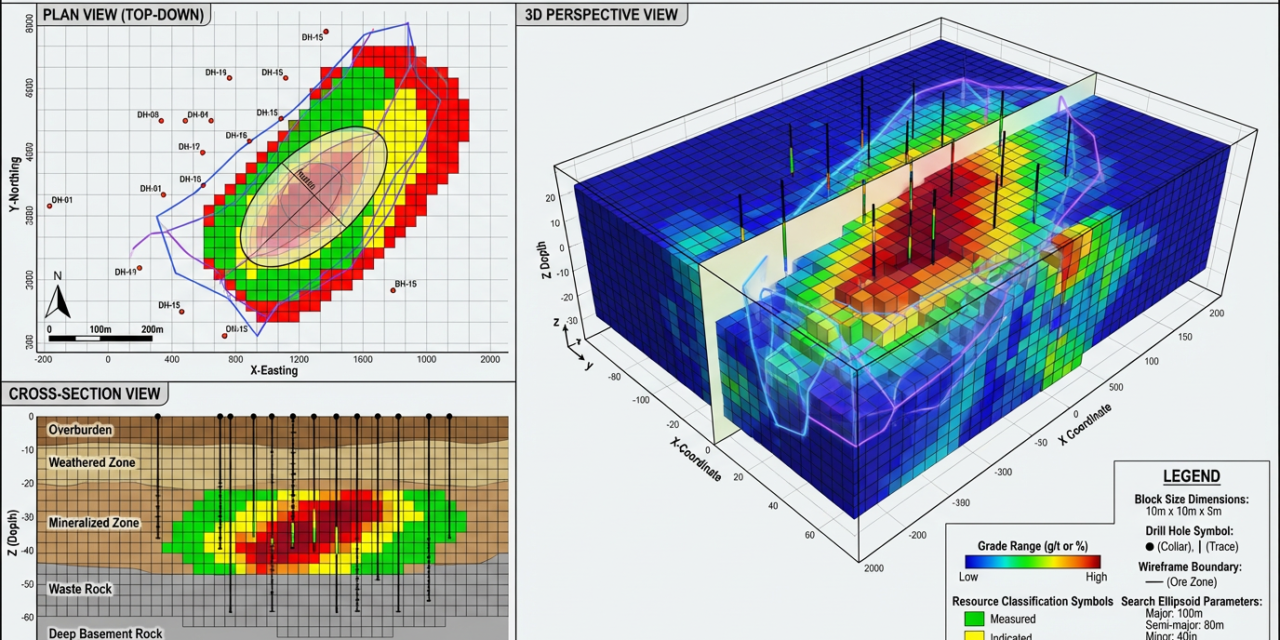
This comprehensive diagram illustrates a complete three-dimensional geological block model with integrated resource classification and grade estimation for a typical mineral deposit. The plan view (top-down, top-left) shows the spatial distribution of resource classification categories across the deposit footprint, with drill hole collar locations marked (DH-01 through DH-16) and systematic grid spacing of 100m × 200m. The color-coded classification scheme displays Measured resources (green blocks) in areas of highest drill density near the deposit center, indicated resources (yellow blocks) in moderately drilled areas, and Inferred resources (red blocks) in sparsely drilled peripheral zones.

The 3D perspective view (top-right) presents the complete block model as a volumetric representation, showing the deposit extending from surface (overburden and weathered zone) through the mineralized zone to deep basement rock. Block dimensions are 10m × 10m × 5m, optimized for the deposit geometry and drill spacing. Drill hole symbols distinguish between collar locations (black dots) and drill traces (vertical lines) penetrating the mineralized zone. The wireframe boundary (ore zone outline) delineates the economic mineralization envelope. The cross-section view (bottom-left) displays the vertical distribution of geological units and resource classification through a representative section, showing overburden (0-10m depth), weathered zone (10-20m), mineralized zone (20-40m), waste rock (40-60m), and deep basement rock (below 60m).

The grade distribution within the mineralized zone ranges from low-grade (blue, 0-2 g/t) through medium-grade (green, 2-4 g/t; yellow, 4-6 g/t) to high-grade (red, 6-10 g/t), with the highest grades concentrated in the central portion of the deposit. The legend (bottom-right) provides complete documentation of block size dimensions, drill hole symbols, wireframe boundaries, grade ranges, resource classification symbols, and search ellipsoid parameters (major axis 100m, semi-major 80m, minor 30m, azimuth 45°, dip 30°). This integrated block model demonstrates how geological interpretation, drill hole data, geostatistical estimation, and resource classification are combined to produce a comprehensive three-dimensional representation of the mineral deposit suitable for resource reporting under SNI 4726-2019 and mine planning applications.

Advantages: Kriging accounts for spatial continuity, sample clustering, and screening effects. It provides optimal (minimum variance) estimates and quantifies estimation uncertainty through kriging variance. Kriging honors the variogram structure and produces smooth, geologically plausible grade distributions [6].

Limitations: Kriging requires variography, which can be time-consuming and subjective. Kriging produces smoothed estimates that underestimate high grades and overestimate low grades (conditional bias). Kriging variance is not a true measure of estimation uncertainty and cannot be used directly for risk analysis [7].

Appropriate Applications: Ordinary kriging is the industry-standard method for resource estimation in most deposit types where data density is adequate and spatial continuity is well-defined [6].

The 3D block model shown in Figure 5 illustrates the result of kriging estimation, with blocks color-coded by estimated grade (blue for low grades, green for medium grades, yellow for high grades, red for very high grades). The plan view (top-left) shows the spatial distribution of grades across the deposit, while the 3D perspective view (top-right) displays the complete volumetric model with drill hole traces and wireframe boundaries. The cross-section view (bottom-left) reveals the vertical distribution of grades through the mineralized zone, demonstrating how kriging produces smooth grade transitions that honor the spatial continuity structure.

3.6.3 Indicator Kriging and Multiple Indicator Kriging (MIK)

Indicator kriging transforms grade data into binary indicators (1 if grade exceeds a threshold, 0 otherwise) and estimates the probability that block grades exceed various thresholds. Multiple indicator kriging uses several thresholds to estimate the complete conditional cumulative distribution function (CCDF) of block grades [6].

Advantages: Indicator kriging is robust to extreme values and skewed grade distributions. It provides probabilistic estimates suitable for risk analysis and optimization. MIK can model complex, multimodal grade distributions [6].

Limitations: Indicator kriging requires more intensive variography (one variogram per threshold). It is computationally expensive and may produce order relation problems (estimated probabilities that violate logical constraints) [6].

Appropriate Applications: Indicator kriging is suitable for deposits with highly skewed grade distributions, significant nugget effects, or complex geological domains where ordinary kriging produces excessive smoothing [6].

3.6.4 Estimation Parameters and Search Strategy

Regardless of the estimation method, several parameters control the estimation process:

Search Ellipsoid: The search ellipsoid defines the volume within which samples are selected for estimating each block. The ellipsoid dimensions and orientation are derived from variogram anisotropy parameters [6].

Minimum and Maximum Samples: Minimum sample requirements (typically 4-8 samples) ensure that estimates are adequately supported. Maximum sample limits (typically 12-24 samples) prevent excessive smoothing and reduce computational cost [6].

Octant Search: Dividing the search ellipsoid into octants and requiring a minimum number of samples per octant (typically 1-2) ensures that samples are distributed around the block rather than clustered on one side [6].

Dynamic Anisotropy: For deposits with variable mineralization orientation (e.g., vein systems), the search ellipsoid orientation may be adjusted dynamically based on local geological structure [6].

3.7 Validation and Classification

Validation confirms that resource estimates are reasonable, unbiased, and consistent with input data and geological understanding. Classification assigns confidence categories (Inferred, Indicated, Measured) based on geological confidence, data density, and estimation quality. SNI 4726-2019 requires that estimates be validated using multiple independent methods and that classification criteria be clearly defined and consistently applied [1], [8].

3.7.1 Visual Validation

Visual validation involves comparing estimated block grades against input sample grades on cross-sections, long-sections, and plan views:

Grade Shells: Contouring estimated grades and overlaying sample locations allows visual assessment of whether estimates honor sample grades and geological trends [1].

Swath Plots: Swath plots compare average estimated grades against average sample grades along slices through the deposit (e.g., by easting, northing, or elevation). Systematic deviations indicate bias [1].

Nearest Neighbor Comparison: Comparing kriged estimates against nearest neighbor estimates (assigning each block the grade of the closest sample) reveals the degree of smoothing introduced by kriging [1].

3.7.2 Statistical Validation

Statistical validation quantifies the agreement between estimates and input data:

Global Mean Comparison: The mean of estimated block grades should approximately equal the mean of declustered sample grades. Significant differences indicate global bias [1].

Grade-Tonnage Curves: Comparing grade-tonnage curves derived from block estimates against curves derived from sample data reveals whether estimates reproduce the grade distribution. Kriging typically produces flatter grade-tonnage curves due to smoothing [1].

Conditional Bias Analysis: Conditional bias plots compare estimated grades against actual grades in different grade ranges. Overestimation of low grades and underestimation of high grades indicates excessive conditional bias [7].

3.7.3 Cross-Validation

Cross-validation removes each sample in turn, re-estimates its location using surrounding samples, and compares the estimate against the actual sample grade:

Mean Error: The average difference between estimated and actual values should be close to zero, indicating unbiasedness [1].

Mean Absolute Error: The average absolute difference quantifies estimation accuracy [1].

Correlation Coefficient: The correlation between estimated and actual values indicates the strength of the relationship. Correlations >0.7 indicate good estimation quality [1].

Slope of Regression: The slope of the regression line between estimated and actual values should be close to 1.0. Slopes <1.0 indicate conditional bias (oversmoothing) [7].

3.7.4 Resource Classification

Resource classification assigns confidence categories based on multiple criteria:

Geological Confidence: Measured resources require detailed geological understanding with closely spaced drilling that confirms continuity. Indicated resources require moderate geological confidence with sufficient drilling to establish continuity. Inferred resources are based on limited data with assumed but not confirmed continuity [8].

Data Density: Measured resources typically require drill spacing of 25-50m. Indicated resources require 50-100m spacing. Inferred resources may be based on 100-200m spacing or extrapolation beyond drilled areas [8].

Estimation Quality: Classification may incorporate kriging variance, kriging efficiency (ratio of kriging variance to prior variance), or slope of regression from cross-validation. However, these metrics should supplement rather than replace geological judgment [8].

Classification Boundaries: Classification boundaries should be smooth and geologically plausible, avoiding abrupt transitions or “checkerboard” patterns that indicate over-reliance on mathematical criteria [5].

The plan view in Figure 5 (top-left) illustrates resource classification, with green blocks representing Measured resources in the densely drilled central area, yellow blocks representing Indicated resources in moderately drilled areas, and red blocks representing Inferred resources in sparsely drilled peripheral zones. This classification pattern reflects both drill density and geological confidence, with smooth transitions between categories.

---

4. Frequently Covered-Up Errors in Mineral Resource Estimation

Despite the availability of sophisticated software, standardized methodologies, and regulatory frameworks, mineral resource estimates frequently contain significant errors that remain undetected until production reconciliation reveals substantial discrepancies. These errors are often “covered up” in the sense that they are concealed within technically sophisticated workflows that superficially appear compliant with best practices [3]. This section identifies the most common hidden errors, explains why they escape detection, and provides diagnostic criteria for identifying them.

Figure 6: Common Hidden Errors in Mineral Resource Estimation

This comprehensive diagram illustrates six categories of frequently overlooked errors that can cause 10-50% variance in mineral resource estimates despite superficial compliance with technical standards. The top-left panel shows selective sampling bias, where preferential sampling of visibly mineralized intervals (right histogram, biased mean = 3.8 g/t) distorts the true grade distribution (left histogram, true mean = 2.5 g/t), potentially inflating resource estimates by 20-50%.

The top-center panel illustrates data entry errors in coordinate systems, comparing correct drill hole coordinates (left, systematic grid pattern) versus transposed X/Y coordinates (right, chaotic pattern with misplaced drill holes), which can invalidate spatial analysis and estimation. The top-right panel demonstrates improper compositing effects, contrasting incorrect arithmetic mean averaging (0.5m + 1.2m + 0.8m + 1.5m = 3.0 g/t, marked with red X) versus correct length-weighted averaging ((0.5×4.0) + (1.2×3.5) + (0.8×2.0) + (1.5×2.5)) / (0.5+1.2+0.8+1.5) = 2.9 g/t, marked with green checkmark), showing how equal weighting of variable-length samples introduces bias. The middle-left panel illustrates hard domain boundary errors, showing incorrect cross-domain estimation (top, where high-grade ore bleeds into low-grade waste causing grade dilution) versus correct domain-restricted estimation (bottom, with sharp boundaries preventing cross-contamination).

The middle-center panel demonstrates kriging smoothing artifacts (checkerboard effect), comparing unrealistic alternating high-low grade patterns (left, kriging artifact with small search radius) versus a corrected smooth model (right, with appropriate search parameters and ellipsoid orientation). The middle-right panel shows bulk density measurement errors, contrasting three methods: dry weight only (underestimate, marked with red X), water displacement method using Archimedes principle (correct, marked with green checkmark), and assumed default value SG = 2.5 (error, marked with red X).

The warning banner emphasizes that these errors can cause ±15-30% tonnage variance. This diagram serves as a diagnostic tool for identifying hidden errors that compromise estimate reliability despite appearing technically sound, enabling competent persons and reviewers to detect and correct these systematic flaws before they impact resource reporting and mine planning decisions.

4.1 Sampling Biases and Selective Sampling

Sampling bias—systematic deviation of sample grades from true in-situ grades—is one of the most damaging and difficult-to-detect errors in resource estimation. The top-left panel of Figure 6 illustrates selective sampling bias, where preferential sampling of visibly mineralized intervals produces a biased grade distribution (right histogram, mean = 3.8 g/t) that significantly overestimates the true grade distribution (left histogram, mean = 2.5 g/t).

4.1.1 Preferential Sampling of High-Grade Zones

Geologists may consciously or unconsciously preferentially sample intervals that appear visibly mineralized while avoiding barren or weakly mineralized zones. This practice, sometimes called “high-grading the drill core,” can inflate resource estimates by 20-50% [3]. The bias is particularly insidious because:

• It is difficult to detect retrospectively without access to unsampled core or detailed core photographs.
• It may be rationalized as “efficient sampling” that focuses resources on economic zones.
• It produces internally consistent datasets that pass standard validation checks [3].

Diagnostic Criteria: Selective sampling can be detected by:

• Comparing sampled intervals against total drilled intervals to identify systematic gaps in sampling.
• Examining core photographs to verify that all mineralized intervals were sampled.
• Comparing sample length distributions against geological logging to identify preferential sampling of specific lithologies [15].

Corrective Actions: Implement mandatory sampling protocols that require complete sampling of all intervals within defined mineralized domains, regardless of visual appearance. Use independent core sampling audits to verify compliance [15].

4.1.2 Sample Loss and Recovery Bias

Differential loss of friable, high-grade material during drilling introduces negative bias that is difficult to quantify. This is particularly problematic in oxide zones, weathered rock, and fault zones where competent material is preferentially recovered while friable material is lost as fines [15].

Diagnostic Criteria: Sample loss bias can be detected by:

• Analyzing core recovery data to identify systematic low recovery in specific lithologies or grade ranges.
• Comparing grades in intervals with high recovery (>95%) against grades in intervals with low recovery (<85%).
• Examining drill cuttings and sludge for evidence of lost high-grade material [15].

Corrective Actions: Use drilling methods appropriate for the material being drilled (e.g., triple-tube core barrels in friable zones). Collect and assay drill cuttings or sludge in low-recovery intervals to quantify lost material [15].

4.2 Data Quality and Data-Handling Errors

Data entry errors, coordinate system mistakes, and database corruption can invalidate resource estimates even when sampling and analytical procedures are flawless. The top-center panel of Figure 6 illustrates coordinate system errors, comparing correct drill hole coordinates (left, systematic grid pattern) versus transposed X/Y coordinates (right, chaotic pattern with misplaced drill holes).

4.2.1 Coordinate System Errors

Coordinate system errors occur when drill hole collar coordinates are recorded in the wrong coordinate system, projected incorrectly, or have transposed X/Y or easting/northing values. These errors can displace drill holes by hundreds of meters, invalidating spatial analysis and estimation [3].

Diagnostic Criteria: Coordinate errors can be detected by:

• Plotting drill hole collars on topographic maps or satellite imagery to verify that locations are geologically plausible.
• Checking for systematic offsets or rotations that indicate projection errors.
• Verifying that collar elevations are consistent with topographic surfaces [3].

Corrective Actions: Implement rigorous coordinate verification procedures, including independent survey of collar locations and cross-checking against topographic data. Use standardized coordinate systems and document all transformations [1].

4.2.2 Assay Database Errors

Transcription errors, sample mix-ups, and database corruption can introduce random or systematic errors into assay data. Common errors include:

• Transposed sample IDs or depths, causing grades to be assigned to wrong locations.
• Missing or duplicated assay records, creating gaps or overlaps in the database.
• Unit conversion errors (e.g., ppm vs. g/t, % vs. g/t) that scale grades by factors of 10 or 100 [3].

Diagnostic Criteria: Database errors can be detected by:

• Checking for missing intervals, overlapping intervals, or out-of-sequence samples.
• Comparing assay databases against original laboratory certificates to detect transcription errors.
• Plotting grades against depth or distance to identify anomalous spikes or gaps [3].

Corrective Actions: Implement automated database validation scripts that check for common errors. Maintain audit trails that document all database modifications. Periodically reconcile databases against original source documents [1].

4.3 Compositing and Support Mistakes

Improper compositing is one of the most common and consequential errors in resource estimation, yet it often escapes detection because composited data appear superficially reasonable. The top-right panel of Figure 6 demonstrates the difference between incorrect arithmetic mean averaging (marked with red X) and correct length-weighted averaging (marked with green checkmark).

4.3.1 Arithmetic Mean Instead of Length-Weighted Mean

Using arithmetic mean averaging for variable-length samples gives equal weight to short and long intervals, introducing bias when grade is correlated with sample length. For example, if high-grade intervals are systematically shorter than low-grade intervals (due to selective sampling or geological controls), arithmetic averaging overestimates the true grade [2].

Example: Consider four samples with lengths and grades:

• 0.5m @ 4.0 g/t
• 1.2m @ 3.5 g/t
• 0.8m @ 2.0 g/t
• 1.5m @ 2.5 g/t

Arithmetic mean: (4.0 + 3.5 + 2.0 + 2.5) / 4 = 3.0 g/t (INCORRECT)

Length-weighted mean: (0.5×4.0 + 1.2×3.5 + 0.8×2.0 + 1.5×2.5) / (0.5+1.2+0.8+1.5) = 2.9 g/t (CORRECT)

While the difference appears small in this example, systematic application of arithmetic averaging across thousands of composites can introduce 5-15% bias [2].

Diagnostic Criteria: Arithmetic averaging can be detected by:

• Comparing composite grades calculated using arithmetic versus length-weighted methods.
• Examining the correlation between sample length and grade to identify systematic relationships.
• Checking compositing scripts or software settings to verify that length-weighting is applied [2].

Corrective Actions: Always use length-weighted averaging for variable-length samples. Document compositing procedures in detail and validate composite grades against raw sample data [2].

4.3.2 Failure to Apply Change-of-Support Corrections

Estimating block grades using point sample statistics without change-of-support correction leads to overestimation of high-grade blocks and underestimation of low-grade blocks. This error is particularly problematic when using indicator kriging or conditional simulation without proper support correction [14].

Diagnostic Criteria: Inadequate change-of-support correction can be detected by:

• Comparing the variance of estimated block grades against the expected block variance calculated from the variogram.
• Examining grade-tonnage curves to identify excessive high-grade tonnage.
• Analyzing conditional bias plots to quantify overestimation of low grades and underestimation of high grades [7], [14].

Corrective Actions: Apply appropriate change-of-support corrections using affine correction, indirect lognormal correction, or discrete Gaussian models. Validate corrected estimates against expected block variance [14].

4.4 Geological and Domain Assumption Errors

Geological modeling errors—particularly inappropriate domain boundaries—can introduce significant bias even when estimation procedures are technically correct. The middle-left panel of Figure 6 illustrates hard domain boundary errors, showing how incorrect cross-domain estimation (top) causes grade dilution by allowing high-grade ore to bleed into low-grade waste, versus correct domain-restricted estimation (bottom) with sharp boundaries.

4.4.1 Cross-Domain Estimation

Allowing samples from one geological domain to influence estimates in adjacent domains (cross-domain estimation) dilutes high-grade domains and inflates low-grade domains. This error is particularly damaging when domains have sharp boundaries (e.g., vein contacts, fault boundaries) that should be treated as impermeable [9].

Diagnostic Criteria: Cross-domain estimation can be detected by:

• Examining estimated grades near domain boundaries to identify gradational transitions where sharp contacts are expected.
• Comparing within-domain grade statistics before and after estimation to quantify dilution.
• Plotting sample search patterns to verify that samples are restricted to the correct domain [9].

Corrective Actions: Implement hard domain boundaries that prevent cross-domain estimation. Use domain indicators or separate estimation runs for each domain. Validate domain boundaries against drilling data [9].

4.4.2 Inappropriate Domain Boundaries

Defining domains based on arbitrary criteria (e.g., grade shells, geometric boundaries) rather than geological features creates artificial boundaries that do not reflect true geological controls on mineralization. This can fragment continuous mineralization into multiple domains or combine geologically distinct zones [9].

Diagnostic Criteria: Inappropriate domains can be detected by:

• Comparing within-domain grade variability against global variability to verify that domains are more homogeneous.
• Examining domain boundaries on cross-sections to verify alignment with geological features.
• Analyzing contact analysis plots to quantify grade contrast across domain boundaries [9].

Corrective Actions: Define domains based on geological features (lithology, alteration, structure) rather than grade. Validate domains using statistical tests (e.g., t-tests, ANOVA) to confirm that domains have distinct grade populations [9].

4.5 Statistical and Estimation Pitfalls

Statistical errors in variography, estimation parameters, and validation can produce estimates that appear technically sophisticated but are fundamentally flawed. The middle-center panel of Figure 6 demonstrates kriging smoothing artifacts (checkerboard effect), comparing unrealistic alternating high-low grade patterns (left) versus a corrected smooth model (right).

4.5.1 Checkerboard Effect and Negative Weights

The checkerboard effect—unrealistic alternating high-low grade patterns in block models—results from inappropriate kriging parameters, particularly search ellipsoids that are too small or oriented incorrectly. This artifact indicates that kriging is assigning negative weights to some samples, violating the fundamental assumption that all samples should contribute positively to estimates [5].

Diagnostic Criteria: Checkerboard effects can be detected by:

• Visual inspection of block models on cross-sections or plan views to identify alternating patterns.
• Examining kriging weights to identify negative values.
• Analyzing kriging efficiency (ratio of kriging variance to prior variance) to identify blocks with poor estimation quality [5].

Corrective Actions: Increase search ellipsoid dimensions, adjust ellipsoid orientation to match variogram anisotropy, or reduce the maximum number of samples per block. Consider using simple kriging or IDW in areas with insufficient data [5].

4.5.2 Misuse of Kriging Variance for Uncertainty Quantification

Kriging variance is often misinterpreted as a measure of estimation uncertainty and used directly for resource classification or risk analysis. However, kriging variance depends primarily on sample configuration (data density and spatial arrangement) and is largely independent of sample grades. Two blocks with identical sample configurations have identical kriging variances regardless of whether the samples are all low-grade or all high-grade [7].

Diagnostic Criteria: Misuse of kriging variance can be detected by:

• Examining the correlation between kriging variance and estimated grades (should be near zero).
• Comparing kriging variance against actual estimation errors from cross-validation (often poorly correlated).
• Checking classification criteria to verify that kriging variance is not the sole classification criterion [7].

Corrective Actions: Use kriging variance as one of multiple classification criteria, supplemented by geological confidence, data density, and cross-validation results. Consider conditional simulation for true uncertainty quantification [7].

4.6 Bulk Density Miscalculations

Bulk density (specific gravity) errors directly scale tonnage estimates and are one of the most common sources of reconciliation failure. The middle-right panel of Figure 6 illustrates three bulk density measurement methods: dry weight only (underestimate), water displacement method (correct), and assumed default value (error).

4.6.1 Inadequate Bulk Density Measurements

Many resource estimates rely on assumed default bulk density values (e.g., SG = 2.5 for all rock types) rather than measured values, introducing 10-30% tonnage errors when actual densities differ from assumptions [12]. Even when measurements are collected, inadequate sample sizes or non-representative sampling can introduce bias.

Diagnostic Criteria: Inadequate bulk density data can be detected by:

• Comparing the number of bulk density measurements against the number of assay samples (should be at least 1:20).
• Examining the spatial and lithological distribution of bulk density samples to verify representativeness.
• Comparing assumed versus measured bulk densities to quantify potential tonnage errors [12].

Corrective Actions: Collect bulk density measurements using water displacement (Archimedes) method on representative samples spanning all lithologies, weathering states, and mineralization styles. Develop bulk density models that assign densities based on lithology and grade rather than using global averages [12].

4.6.2 Incorrect Bulk Density Measurement Methods

Using dry weight only (without accounting for porosity) or wax-coating methods (which add weight) can introduce systematic errors. The water displacement method, which measures the volume of water displaced by a sample and calculates density as mass/volume, is the industry standard [12].

Diagnostic Criteria: Incorrect methods can be detected by:

• Reviewing bulk density measurement procedures to verify that water displacement method is used.
• Comparing bulk densities measured using different methods to identify systematic differences.
• Examining bulk density versus porosity relationships to verify physical plausibility [12].

Corrective Actions: Standardize bulk density measurement procedures using water displacement method. Measure both dry and saturated densities to account for porosity effects. Validate bulk density models against independent measurements [12].

---

5. Comprehensive Inspection Checklists Aligned with SNI 4726-2019

This section provides detailed inspection checklists designed to systematically verify that mineral resource investigations meet SNI 4726-2019 requirements and international best practices. The checklists are organized into seven categories corresponding to the major components of the investigation methodology: data validation and metadata, assay and QA/QC, compositing and data preparation, geological modeling, variography and spatial analysis, estimation and validation, and documentation and reporting.

This comprehensive inspection checklist infographic provides a systematic framework for verifying compliance with SNI 4726-2019 standards and established QA/QC protocols for mineral resource estimation. The checklist is organized into seven critical verification categories, each with weighted importance:

(1) Data Validation & Database QC (40% weight) verifies drill hole collar coordinates, survey data validation, assay database integrity, geological logging consistency, chain of custody documentation, and flags missing or invalid coordinate systems as stop-work triggers;

(2) Assay QA/QC Protocols (30% weight) confirms certified reference materials fall within ±2SD limits, field duplicates show HARD <20%, lab duplicates demonstrate acceptable precision, blank contamination remains below detection limits, outlier investigation is documented, and flags >10% QA/QC failures as stop-work triggers;

(3) Compositing & Data Preparation (20% weight) ensures composite length is justified and documented, length-weighted averaging is applied correctly, top-cutting/capping analysis is completed, change of support effects are evaluated, grade distribution is validated, and flags arithmetic mean usage (incorrect method) as a stop-work trigger;

(4) Geological Modeling (10% weight) verifies domain boundaries are geologically justified, cross-sections are validated with drilling data, wireframe quality is checked for overlaps, lithological contacts are honored, hard versus soft boundaries are documented, and flags cross-domain estimation as a stop-work trigger;

(5) Variography & Spatial Analysis (5% weight) confirms experimental variograms are calculated, anisotropy directions are determined, range and sill parameters are documented, variogram models are fitted and validated, search ellipsoid parameters are justified, and flags default/assumed variograms as stop-work triggers; (6) Estimation & Validation (0% weight) ensures estimation method is documented (kriging/ID2), block size optimization is performed, visual validation with grade shells is reviewed, statistical validation includes swath plots and Q-Q plots, nearest neighbor analysis is completed, smoothing effects are quantified, and flags no validation performed as a stop-work trigger; (7) Documentation & Reporting (0% weight) verifies estimation parameters are recorded, assumptions and limitations are stated, SNI 4726-2019 compliance is confirmed, competent person sign-off is obtained, audit trail is maintained, and flags incomplete documentation as a stop-work trigger.

The legend distinguishes between standard checklist items (white boxes), critical control points (yellow warning triangles), and stop-work triggers (red circles). The bottom section provides signature lines for Inspector Approval, Senior Geologist Approval, and QP (Qualified Person) Approval with dates, along with a certification statement confirming compliance with SNI 4726-2019 standards and established QA/QC protocols.

This checklist serves as a comprehensive verification tool for competent persons, technical reviewers, and regulatory auditors to ensure that mineral resource estimates are technically sound, defensible, and compliant with Indonesian national standards.

Each checklist category includes:

• Standard verification items: Routine checks that should be performed for all resource estimates.
• Critical control points: High-risk items that require particular attention and senior review.
• Stop-work triggers: Fatal flaws that invalidate the estimate and require immediate corrective action.

The checklists are designed to be used iteratively throughout the investigation workflow, with early-stage checks (data validation, QA/QC) performed before proceeding to later stages (estimation, classification). This approach prevents the propagation of errors through the workflow and reduces rework.

5.1 Data Validation and Metadata Checklist

Objective: Verify that exploration data are complete, accurate, and adequately documented to support resource estimation.

Drill Hole Database Verification (Weight: 40%)

•  Collar coordinates verified: All drill hole collar coordinates have been independently surveyed using differential GPS or total station methods with documented accuracy (±0.5m horizontal, ±0.1m vertical).
•  Survey data validated: Downhole survey data (azimuth, dip) have been collected at appropriate intervals (≤30m) using gyroscopic or magnetic survey tools. Survey data have been validated for internal consistency and physical plausibility.
•  Assay database integrity checked: Assay database has been checked for missing intervals, overlapping intervals, out-of-sequence samples, negative values, and physically implausible grades. All anomalies have been investigated and resolved.
•  Geological logging consistency reviewed: Geological logging codes are consistent across all drill holes. Logging has been performed by qualified geologists using standardized procedures. Core photographs are available for all mineralized intervals.
•  ⚠️ Chain of custody documentation complete: Sample collection, transport, and storage procedures are documented. Chain of custody forms are complete for all samples. Sample security measures are adequate for the commodity value.
•  🛑 Missing or invalid coordinate systems: Coordinate system is clearly defined and documented. All spatial data use consistent coordinate systems. Coordinate transformations are documented and validated.

Diagnostic Questions:

• Are collar coordinates consistent with topographic surfaces and geological maps?
• Do downhole surveys show physically plausible trajectories without abrupt changes?
• Are there systematic gaps in the assay database that indicate selective sampling?

5.2 Assay and QA/QC Checklist

Objective: Verify that analytical data are accurate, precise, and suitable for resource estimation.

Analytical Methods and Detection Limits (Weight: 30%)

•  Analytical methods appropriate: Analytical methods (fire assay, ICP-MS, XRF) are appropriate for the commodity, expected grade range, and mineralogical characteristics. Detection limits are below economic cutoff grades.
•  CRM/Reference materials within ±2SD: Certified reference materials have been inserted at a frequency of ≥5% (1 in 20 samples). CRM results fall within ±2 standard deviations of certified values for ≥95% of insertions.
•  Field duplicates HARD <20%: Field duplicates have been collected at a frequency of ≥5%. Half Absolute Relative Difference (HARD) between duplicate pairs is <20% for ≥90% of pairs.
•  Lab duplicates precision acceptable: Laboratory duplicates have been prepared at a frequency of ≥5%. HARD between duplicate pairs is <10% for ≥90% of pairs.
•  Blank contamination <detection limit: Blank samples have been inserted at a frequency of ≥5%. Blank results are below detection limits for ≥95% of insertions.
•  ⚠️ Outlier investigation documented: High-grade outliers (>3 standard deviations from mean) have been investigated. Re-assays or check assays have been performed where appropriate. Outlier treatment (top-cutting, capping) is documented and justified.
•  🛑 >10% QA/QC failures: If >10% of QA/QC samples fail acceptance criteria, the affected sample batches must be re-assayed or rejected. Root cause analysis must be performed to identify and correct systematic problems.

Diagnostic Questions:

• Do CRM control charts show systematic bias or drift over time?
• Are blank failures associated with specific sample batches or high-grade samples?
• Do field duplicate HARD values increase with grade, indicating nugget effect?

5.3 Compositing and Data Preparation Checklist

Objective: Verify that sample compositing preserves grade distributions and is appropriate for the estimation method.

Compositing Strategy (Weight: 20%)

•  Composite length justified and documented: Composite length is appropriate for minimum mining selectivity, geological continuity, and data density. Composite length is typically 1/3 to 1/2 of drill spacing.
•  Length-weighted averaging applied correctly: Variable-length samples have been composited using length-weighted averaging. Compositing scripts or software settings have been validated.
•  Top-cutting/capping analysis completed: High-grade outliers have been identified using statistical methods (probability plots, coefficient of variation). Top-cut thresholds are documented and justified. Impact of top-cutting on mean grade and tonnage is quantified.
•  ⚠️ Change of support effects evaluated: Change-of-support corrections have been applied or evaluated. Block variance is expected to be lower than sample variance by a factor consistent with block size and variogram parameters.
•  Grade distribution validated: Composite grade distribution has been compared against raw sample distribution. Mean, variance, and coefficient of variation are consistent. Histograms and probability plots show expected characteristics.
•  🛑 Arithmetic mean used (incorrect): If arithmetic mean averaging has been used for variable-length samples, compositing must be redone using length-weighted averaging. Impact on resource estimate must be quantified.

Diagnostic Questions:

• Does composite length honor geological boundaries without creating excessive residual intervals?
• Are high-grade composites spatially clustered or randomly distributed?
• Does the composite grade distribution show realistic characteristics for the deposit type?

5.4 Geological Modeling Checklist

Objective: Verify that geological models are based on sound interpretation and adequately constrain resource estimation.

Domain Definition and Wireframe Quality (Weight: 10%)

•  Domain boundaries geologically justified: Geological domains are defined based on lithology, alteration, mineralization style, or structural controls. Domain boundaries align with observable geological features.
•  Cross-sections validated with drilling: Geological interpretations on cross-sections are consistent with drill hole logging. Interpretations are supported by adequate drill density.
•  Wireframe quality checked (no overlaps): Wireframe surfaces are closed, non-overlapping, and topologically valid. Wireframe quality has been checked using automated validation tools.
•  Lithological contacts honored: Estimation domains honor lithological contacts and do not arbitrarily cut across geological boundaries.
•  ⚠️ Hard boundaries vs soft boundaries documented: Treatment of domain boundaries (hard vs. soft) is documented and justified based on geological characteristics and grade contrast.
•  🛑 Cross-domain estimation detected: If samples from one domain are influencing estimates in adjacent domains, estimation parameters must be revised to enforce hard boundaries or domain-restricted estimation.

Diagnostic Questions:

• Are domain boundaries smooth and geologically plausible, or do they show artifacts of interpretation bias?
• Do domains have sufficient data density to support independent estimation?
• Are grade distributions more homogeneous within domains than globally?

5.5 Variography and Spatial Analysis Checklist

Objective: Verify that variography appropriately characterizes spatial continuity and supports estimation parameters.

Variogram Modeling (Weight: 5%)

•  Experimental variograms calculated: Experimental variograms have been calculated in multiple directions to assess anisotropy. Lag spacing and number of lags are appropriate for data density and deposit size.
•  Anisotropy directions determined: Principal directions of continuity (major, semi-major, minor axes) have been identified. Anisotropy ratios are documented.
•  Range and sill parameters documented: Variogram parameters (nugget, sill, range) are documented for each direction. Nugget effect is <50% of total sill.
•  Variogram model fitted and validated: Theoretical variogram models (spherical, exponential, Gaussian) have been fitted to experimental variograms. Model fit quality is acceptable (visual inspection and cross-validation).
•  ⚠️ Search ellipsoid parameters justified: Search ellipsoid dimensions and orientation are derived from variogram parameters. Ellipsoid dimensions are typically 1.5-2.0 times variogram ranges.
•  🛑 Default/assumed variogram used: If default or assumed variogram parameters have been used without experimental variography, variograms must be calculated from actual data. Impact on resource estimate must be quantified.

Diagnostic Questions:

• Do experimental variograms show clear spatial structure, or are they dominated by nugget effect?
• Are variogram ranges consistent with drill spacing and geological continuity?
• Do directional variograms show anisotropy consistent with geological structure?

5.6 Estimation and Validation Checklist

Objective: Verify that estimation methods are appropriate and that estimates are validated using multiple independent methods.

Estimation Parameters and Validation (Weight: 0%)

•  Estimation method documented (kriging/ID2): Estimation method (ordinary kriging, inverse distance, indicator kriging) is documented and justified based on deposit characteristics and data density.
•  Block size optimization performed: Block dimensions are appropriate for minimum mining selectivity and data density. Block discretization (sub-blocking) is used near domain boundaries.
•  Visual validation (grade shells reviewed): Estimated block grades have been visually compared against input sample grades on cross-sections and plan views. Grade shells and contours are geologically plausible.
•  Statistical validation (swath plots, Q-Q plots): Swath plots compare average estimated grades against average sample grades along slices through the deposit. Quantile-quantile plots compare estimated and sample grade distributions.
•  Nearest neighbor analysis completed: Nearest neighbor estimates have been compared against kriged estimates to quantify smoothing effects.
•  ⚠️ Smoothing effects quantified: Conditional bias has been quantified using conditional bias plots or slope of regression from cross-validation. Excessive smoothing (slope <0.7) has been investigated.
•  🛑 No validation performed: If no validation has been performed, estimates cannot be accepted. Multiple independent validation methods must be applied before estimates are used for resource reporting.

Diagnostic Questions:

• Do swath plots show systematic deviations between estimated and sample grades?
• Are estimated block grades consistent with sample grades in densely drilled areas?
• Does cross-validation show acceptable correlation (>0.7) and low bias?

5.7 Documentation and Reporting Checklist

Objective: Verify that all procedures, assumptions, and results are adequately documented to support independent technical review and regulatory compliance.

Documentation Completeness (Weight: 0%)

•  Estimation parameters recorded: All estimation parameters (search ellipsoid, minimum/maximum samples, octant search, top-cuts, bulk density) are documented in a format suitable for independent review.
•  Assumptions and limitations stated: Key assumptions (geological continuity, grade distribution, metallurgical recovery) and limitations (data density, geological uncertainty) are clearly stated.
•  SNI 4726-2019 compliance confirmed: Resource estimate complies with SNI 4726-2019 requirements for data quality, geological understanding, estimation methodology, classification criteria, and validation.
•  Competent Person sign-off obtained: A qualified Competent Person has reviewed and approved the resource estimate. Competent Person’s qualifications and professional affiliations are documented.
•  ⚠️ Audit trail maintained: All data processing steps, estimation runs, and validation analyses are documented with version control. Original data and intermediate results are archived.
•  🛑 Incomplete documentation: If documentation is insufficient to support independent technical review, additional documentation must be prepared before the estimate can be used for public reporting or investment decisions.

Diagnostic Questions:

• Can an independent reviewer reproduce the resource estimate using the documented procedures?
• Are all material assumptions and limitations clearly disclosed?
• Does the documentation provide sufficient transparency for regulatory compliance?

---

6. Conclusion

Reliable mineral resource estimation requires disciplined application of rigorous methodologies, systematic detection and correction of errors, and transparent documentation that supports independent technical review. This report has presented a comprehensive framework for conducting mineral resource investigations that produce estimates compliant with SNI 4726-2019 and international reporting standards.

The investigation methodology presented in Section 3 emphasizes that reliable estimates depend on:

1. Systematic sampling with robust QA/QC programs that detect and correct analytical errors, sampling bias, and data quality problems before they propagate through the estimation workflow [1], [11], [15].
2. Appropriate compositing and change-of-support corrections that preserve grade distributions and account for the fundamental difference between point sample grades and block grades [2], [14].
3. Geologically justified domain definitions that honor lithological boundaries, structural controls, and mineralization styles while avoiding arbitrary grade-based domains [9].
4. Rigorous variography that quantifies spatial continuity and anisotropy, providing the foundation for optimal sample weighting during kriging [1].
5. Validation using multiple independent methods that confirm estimates are unbiased, consistent with input data, and geologically plausible [1], [7].

The analysis of frequently covered-up errors in Section 4 demonstrates that many superficially correct estimates conceal critical flaws including selective sampling bias, improper compositing, cross-domain estimation, checkerboard artifacts, and bulk density miscalculations. These errors can introduce 10-50% variance in resource tonnage and grade estimates, potentially rendering projects economically unviable [3], [12], [15]. The diagnostic criteria and corrective actions provided enable competent persons and reviewers to detect and correct these systematic flaws.

The comprehensive inspection checklists in Section 5 provide a systematic framework for verifying compliance with SNI 4726-2019 requirements across seven critical categories: data validation, assay QA/QC, compositing, geological modeling, variography, estimation and validation, and documentation. The weighted checklist structure prioritizes high-risk items (data validation 40%, assay QA/QC 30%, compositing 20%) while ensuring that all components receive appropriate scrutiny.

Key recommendations for mining professionals and competent persons responsible for mineral resource estimation in Indonesia include:

Implement Mandatory QA/QC Protocols: Establish comprehensive QA/QC programs with certified reference materials, blank samples, and field duplicates at frequencies sufficient to provide statistical confidence (≥5% insertion rates). Monitor laboratory performance using control charts and trigger corrective actions when acceptance criteria are not met [11].

Enforce Complete Sampling Protocols: Require complete sampling of all intervals within defined mineralized domains to prevent selective sampling bias. Use independent core sampling audits to verify compliance [15].

Apply Length-Weighted Compositing: Always use length-weighted averaging for variable-length samples. Validate compositing procedures and quantify the impact of top-cutting on mean grade and tonnage [2].

Define Geologically Justified Domains: Base domain definitions on geological features (lithology, alteration, structure) rather than grade. Validate domains using statistical tests and ensure adequate data density for independent estimation [9].

Perform Rigorous Validation: Apply multiple independent validation methods including visual inspection, swath plots, cross-validation, and nearest neighbor comparison. Quantify conditional bias and smoothing effects [1], [7].

Maintain Transparent Documentation: Document all procedures, assumptions, limitations, and validation results in a format that supports independent technical review and regulatory compliance. Maintain audit trails with version control [1].

The framework presented in this report provides mining professionals with actionable procedures, critical control points, and decision criteria to ensure that exploration results translate into reliable, defensible mineral resource estimates suitable for investment decisions, mine planning, and regulatory compliance under SNI 4726-2019. By systematically applying these methodologies and verification protocols, the Indonesian mining industry can enhance the reliability of resource estimates, reduce reconciliation failures, and strengthen investor confidence in reported mineral resources.

---

7. References

[1] Pressacco, R., Srivastava, R. M., & Abzalov, M. (2024). Some common flaws encountered in mineral resource estimation and how to avoid them. CIM Journal. https://doi.org/10.1080/19236026.2024.2322391

[2] Abzalov, M. (2025). Compositing High Resolution Assay Data for Mineral Resources. https://doi.org/10.7939/81887

[3] Pressacco, R., Srivastava, R. M., & Abzalov, M. (2024). Some common flaws encountered in mineral resource estimation and how to avoid them. CIM Journal. https://doi.org/10.1080/19236026.2024.2322391

[4] Indonesia Post-Pandemic Outlook: Strategy towards Net-Zero Emissions by 2060 from the Renewables and Carbon-Neutral Energy Perspectives. (2022). https://doi.org/10.55981/brin.562

[5] Pressacco, R., & Srivastava, R. M. (2021). The checkerboard effect and mineral resource reporting of underground mineral resources. CIM Journal. https://doi.org/10.1080/19236026.2021.1902203

[6] Haldar, S. K. (2013). Chapter 8 – Mineral Resource and Ore Reserve Estimation. https://doi.org/10.1016/B978-0-12-416005-7.00008-8

[7] Nowak, M., Leuangthong, O., & Ortiz, J. M. (2017). Conditional Bias in Kriging: Let’s Keep It. https://doi.org/10.1007/978-3-319-46819-8_20

[8] Noppé, M. (2014). Communicating confidence in Mineral Resources and Mineral Reserves. Journal of The South African Institute of Mining and Metallurgy.

[9] Emery, X., & Ortiz, J. M. (2005). Estimation of mineral resources using grade domains: critical analysis and a suggested methodology. Journal of The South African Institute of Mining and Metallurgy.

[10] Yamamoto, J. K. (1999). Quantification of Uncertainty in Ore-Reserve Estimation: Applications to Chapada Copper Deposit, State of Goiás, Brazil. Natural Resources Research, 8(3). https://doi.org/10.1023/A:1021894703729

[11] Gursuren, T., Tercan, A. E., & Hindistan, M. A. (2023). How does better quality data affect the value of a mining project? https://doi.org/10.22353/.v16i1.2267

[12] Dominy, S. C., Annels, A. E., Johansen, G. F., & Cuffley, B. W. (2002). Errors and Uncertainty in Mineral Resource and Ore Reserve Estimation: The Importance of Getting it Right. Exploration and Mining Geology, 11(1-4), 77-98. https://doi.org/10.2113/11.1-4.77

[13] Aswadi, A. (2023). Estimasi sumberdaya nikel mengunakan metode inverse distance weight pt ang and fang brothers. JGE, 9(1). https://doi.org/10.23960/jge.v9i1.235

[14] Janas, D. (2001). Change of support correction in mineral resource estimation.

[15] Minnitt, R. C. A. (2018). The costs of sampling errors and bias to the mining industry. Journal of The South African Institute of Mining and Metallurgy, 118(8). https://doi.org/10.17159/2411-9717/2018/V118N8A1

[18] Downing, B. W., Giroux, G. H., & Vann, J. (2025). Some basic improvements in mineral resource estimation and reporting. CIM Journal. https://doi.org/10.1080/19236026.2024.2430154

[19] Lock, N. P. (2020). RPEEE (Reasonable Prospects for Eventual Economic Extraction): The critical core to the SAMREC Code. Journal of The South African Institute of Mining and Metallurgy, 116(7). https://doi.org/10.17159/2411-9717/1240/2020

[20] Conoras, H. (2017). Klasifikasi sumberdaya endapan nikel laterit daerah pulau obi, halmahera selatan dengan pendekatan relative kriging standard deviation (rksd).

[21] Estimasi Sumberdaya Bauksit Menggunakan Metode Geostatistik di PT. XYZ Kabupaten Mempawah. (2022). https://doi.org/10.29313/jrtp.v2i2.1141

[22] Giurco, D., Prior, T., Mudd, G., Mason, L., & Behrisch, J. (2010). Peak Minerals in Australia: a review of changing impacts and benefits.

[23] Jowitt, S. M., Mudd, G. M., & Thompson, J. F. H. (2025). Mineral Resources and Reserves: Their Estimation, Use, and Abuse. https://doi.org/10.5382/com.16.13

[29] Budiman, H., Slamet, A., Wibisono, G., Zaharim, A., & Sopyan, I. (2022). Toward building local capacity: Progress on the providing of certified calibration gas mixtures. Nucleation and Atmospheric Aerosols. https://doi.org/10.1063/5.0108283

[30] Fourie, P. J., & Dohm, C. (2016). Review of gold reef sampling and its impact on the mine call factor. Journal of The South African Institute of Mining and Metallurgy, 116(11). https://doi.org/10.17159/2411-9717/2016